SHAP-guided explanations
Adding SHAP to the explainer will make LUX try to build the explanation tree that is consistent with SHAP values. In some cases this is important feature, especially when the model is analysed not only with LUX, but also with SHAP.
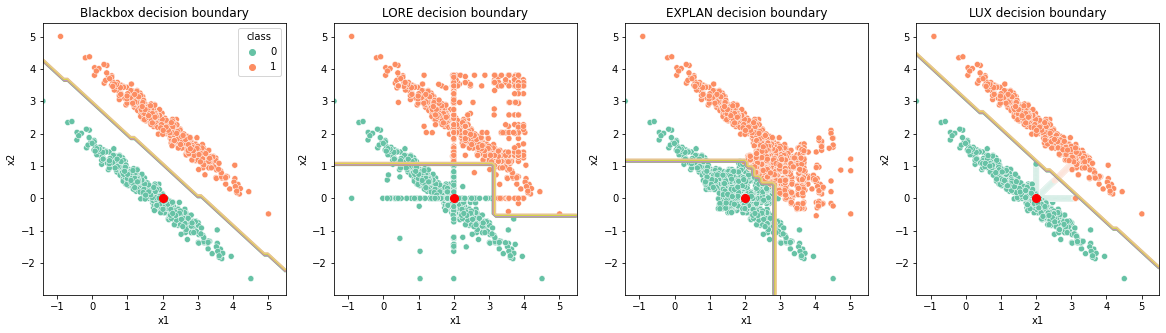
It also helps reducing so called Rashomon effect, because the LUX model uses the same features as blackbox model and therefore the explanations are suppose to be compliant with what really is happening in the balckbox model. This is done via SHAP-guided sampling method that generates the samples in the direction of the decision boundary of a blackbox model, but also due to oblique splits that can handle the linear boundaries better. The example of the situation is visualized in the below figure, where you can observe how others’ explainers decision boundary differ with respect to the balckbox decision boundary. LUX maintains the similar behaviour to the balckbox model, limiting the Rashomon effect.
Tutorials demonstrating the Rashomon effect:
The full example (shown below) with multiple datasets can be found here: Notebook
Another example of this phenomenon was given here: XOR problem where we demonstrate how the greedy nature of the decision tree algorithm can be overcome with SHAP-sampling, also limiting the Rashomon effect.
Loading the dataset and building explanations without SHAP support
For the sake of simplicity we use Wine dataset. Below there is a code that loads the dataset and fits RandomForestClassifier to it.
from sklearn.ensemble import RandomForestClassifier
from lux.lux import LUX
from sklearn import datasets
from sklearn.model_selection import train_test_split
import numpy as np
import pandas as pd

wine = datasets.load_wine()
features = wine['feature_names']
target = 'class'
rs=42
fraction=0.01

#create daatframe with columns names as strings (LUX accepts only DataFrames withj string columns names)
df_wine = pd.DataFrame(wine.data,columns=features)
df_wine[target] = wine.target

#train classifier
train, test = train_test_split(df_wine, random_state=rs)
clf = RandomForestClassifier(random_state=42)#svm.SVC(probability=True, random_state=rs)
clf.fit(train[features],train[target])
clf.score(test[features],test[target])
Explanation without SHAP-guided explanations
Once we ha a model, we can explain it. First, we are going to explain it without SHAP-support. Below there is a code that fits LUX, and shows the visualization of the explanation.
import graphviz
import graphviz
from graphviz import Source
from IPython.display import SVG, Image
i2e = train[features].sample(1, random_state=42).values
#train lux on neighbourhood equal 30% instances
lux = LUX(predict_proba = clf.predict_proba, neighborhood_size=int(len(train)*fraction),max_depth=2, node_size_limit = 1, grow_confidence_threshold = 0 )
lux.fit(train[features], train[target], instance_to_explain=i2e,class_names=[0,1,2])
i2edf = pd.DataFrame(i2e, columns=features)
i2edf[target] =clf.predict(i2edf.values.reshape(1,-1))[0]
lux.uid3.tree.save_dot('tree-wine.dot',fmt='.2f',visual=True, background_data=train, instance2explain=i2edf)
gvz=graphviz.Source.from_file('tree-wine.dot')
!dot -Tpng tree-wine.dot > tree-wine.png
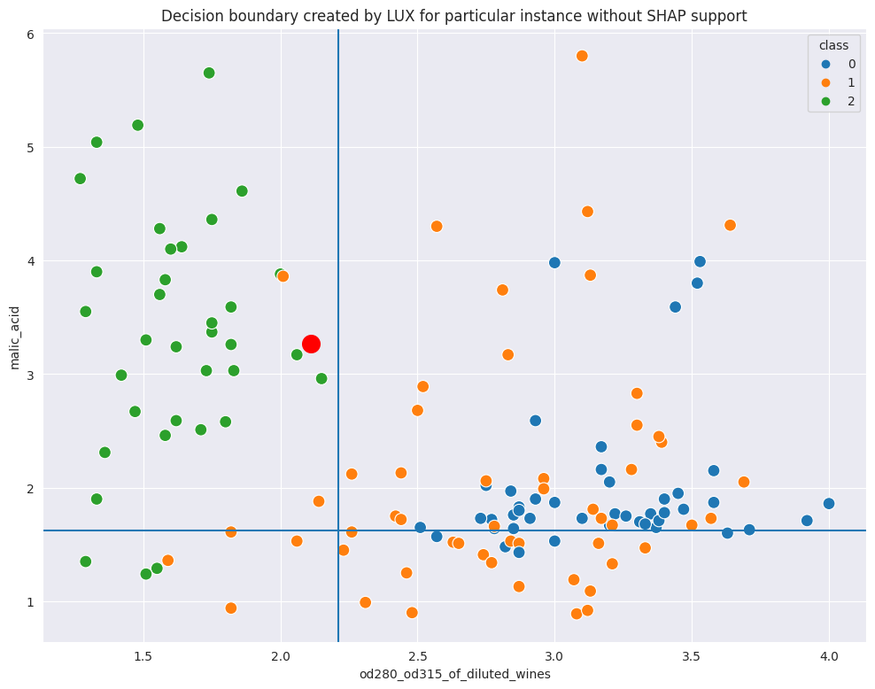
Image('tree-wine.png')
Whn you look at the scatterplot with decision boundaries marked, you can see that it is reasonable, but can we get better?
Explanation with SHAP-guided explantions
Note, that to enable SHAP-guided explanations, you only need to pass classifier as a parameter to LUX.
lux = LUX(predict_proba = clf.predict_proba, classifier=clf, neighborhood_size=int(len(train)*fraction),max_depth=2, node_size_limit = 3, grow_confidence_threshold = 0 )
lux.fit(train[features], train[target], instance_to_explain=iris_instance,class_names=[0,1,2],discount_importance=False)
i2edf = pd.DataFrame(i2e, columns=features)
i2edf[target] =clf.predict(i2edf.values.reshape(1,-1))[0]
lux.uid3.tree.save_dot('tree-wine-shap.dot',fmt='.2f',visual=True, background_data=train, instance2explain=i2edf)
gvz=graphviz.Source.from_file('tree-wine-shap.dot')
!dot -Tpng tree-wine-shap.dot > tree-wine-shap.png
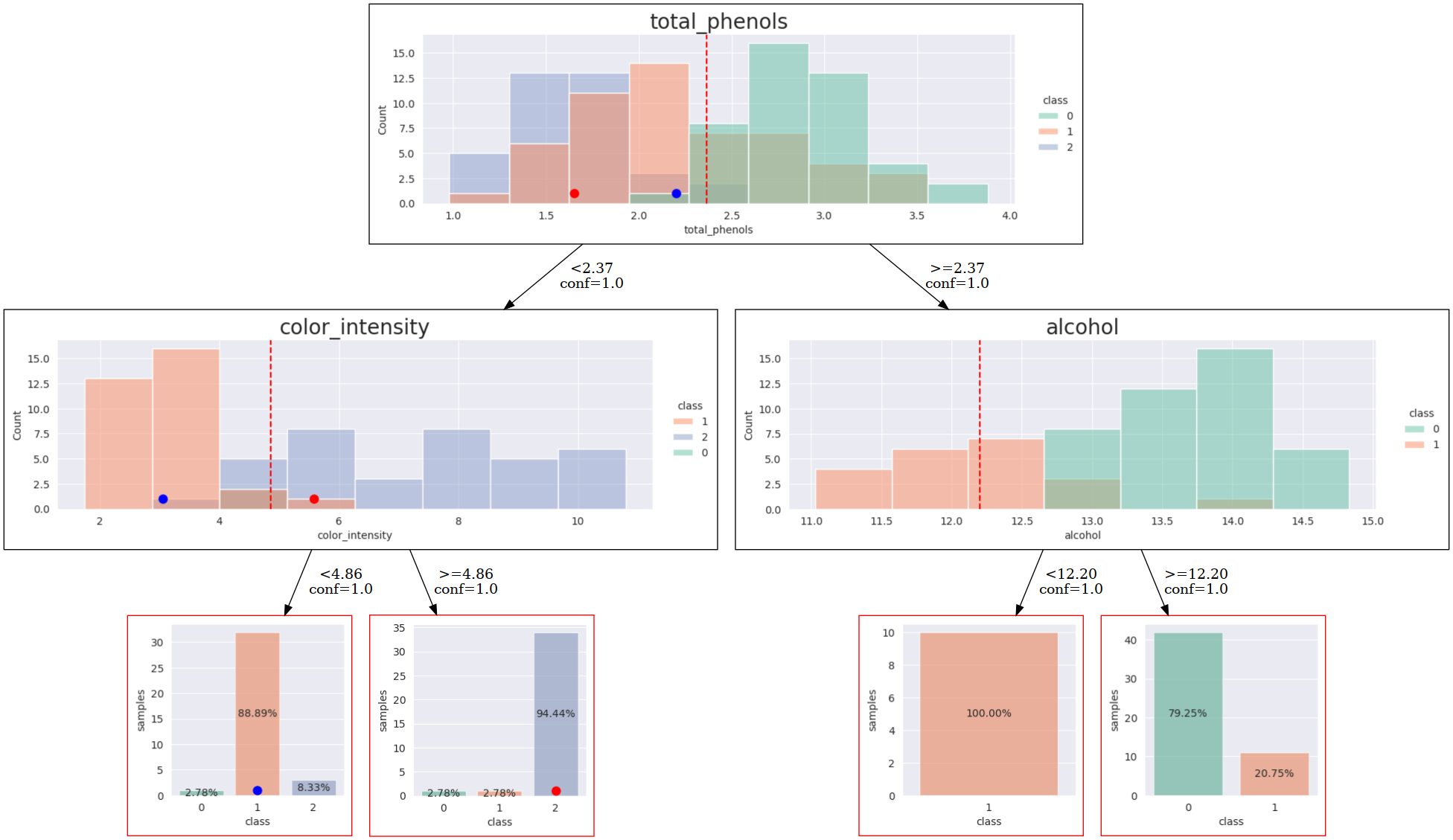
Image('tree-wine-shap.png')
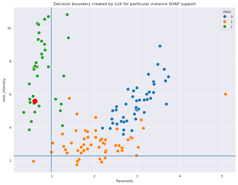
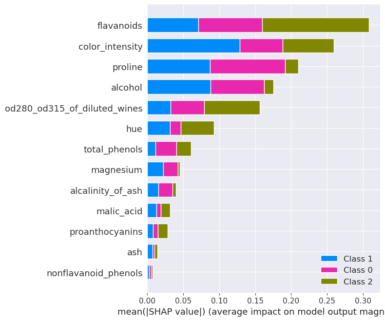
Now, first look at the SHAP values generated separately for the model. One can observe, that there are two features that contribute most tyo the models decisions. These are not the features selected in previous step. However, when we run the visualization again, for the LUX with SHAP-guided explanations, we ge the following decision tree. It is clear that the explanation model is now in compliance with balckbox classifier with respect to features used fro explanations.
The explanation tree is shown below. You can see that it is better aligned with SHAP-value than the pure decision tree generated without SHAP-guidance.
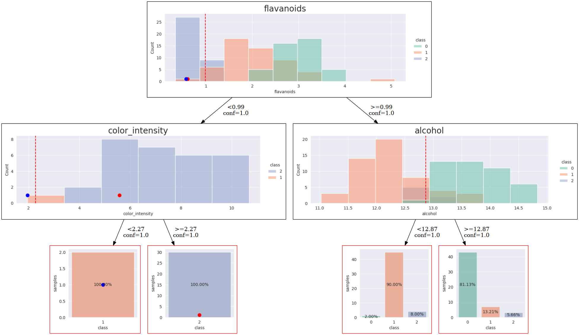
When you compare the scatterplot with decision boundaries from the previous one, you will also observe, that the SHAP-guided version is more clear: